Designing URLLC via nonasymptotic information theory–part 4

An updated and expanded version of these notes can be found here

In part 3 we learnt how to evaluate the achievability bound, i.e., the blue curve in the figure below.

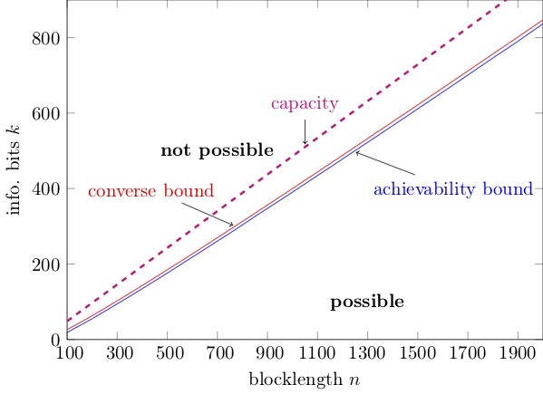
This post is about computing the red curve, i.e., the converse bound.

Converse bounds in information theory express an impossibility condition. In our case, a converse result says that no $(k,n,\epsilon)$-code can be found for which the triplets $(k,n,\epsilon)$ violate a certain relation. Converse bounds give an upper bound on $k^\star(n,\epsilon)$ and hence on $R^\star(k,n)$. Equivalently, they give a lower bound on $\epsilon^\star(k,n)$.

I will review in this post a very general technique to obtain converse bounds in finite-blocklength information theory, which relies on the so-called metaconverse theorem ¹.

Before introducing the metaconverse theorem, we need to review some basic concepts in binary hypothesis testing.

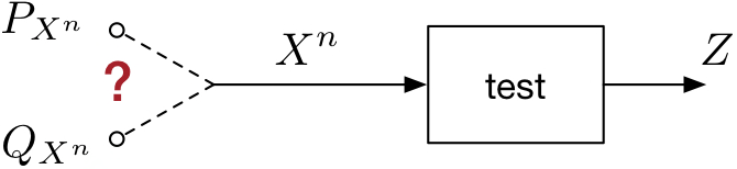
Binary hypothesis testing deals with the following problem (see figure below). We observe a vector $X^n$ which may have been generated according to a distribution $P_{X^n}$ or according to an alternative distribution $Q_{X^n}$. Our task is to discover which of the two distributions generated $X^n$.

To do so, we design a test $Z$ whose input is the vector $X^n$ and whose output is a binary value ${0,1}$. We use the convention that $0$ indicates that the test chooses $P_X^{n}$ and $1$ indicates that the test chooses $Q_{X^n}$.

We can think of the test $Z$ as a binary partition of the set of the vectors $X^n$.

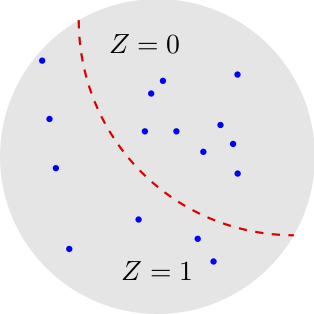
Actually, we will need the more general notion of randomized test, in which the test is a conditional distribution $P_{Z|X^n}$. Coarsely speaking, for some values of $X^n$, we may flip a coin to decide whether $Z=0$ or $Z=1$.

We are interested in the test that minimizes the probability of misclassification when $X^n$ is generated according to $Q_{X^n}$ given that the probability of correct classification under $P_{X^n} $ is above a given target. Mathematically, we define the probability of misclassification under $Q_{X^n}$ as

\[Q_{X^n}[Z=0]=\sum_{x^n}Q_{X^n}(x^n)P_{Z | X^n}(0 | x^n).\]

To parse this expression, recall that $Z=0$ means that the test chooses $P_{X^n}$, which is the wrong distribution in this case. Here, I assumed for simplicity that $X^n$ is a discrete random variable. For the continuous case, one needs to replace the sum with an integral. The probability of correct classification under $P_{X^n}$ is similarly given by

\[P_{X^n}[Z=0]=\sum_{x^n}P_{X^n}(x^n)P_{Z | X^n}(0 | x^n).\]

We let $\beta_{\alpha}(P_{X^n},Q_{X^n})$ be the Neyman-Pearson beta function, which denotes the smallest possible misclassification probability under $Q_{X^n}$ when the probability of correct classification under $P_{X^n}$ is at least $\alpha$:

\[\beta_{\alpha}(P_{X^n},Q_{X^n})=\inf_{P_{Z| X^n}: P_{X^n}[Z=0]\geq \alpha} Q_{X^n}[Z=0].\]

It follows from the Neyman-Pearson lemma (see e.g., p. 144 of the following lecture notes) that $\beta_{\alpha}(P_{X^n},Q_{X^n})$ is achieved by the test that computes the log-likelihood $\log \frac{P_{X^n}(x^n)}{Q_{X^n}(x^n)}$ and sets $Z=0$ if the log-likelihood is above a threshold $\gamma$; it sets $Z=1$ otherwise. Here, $\gamma$ is chosen so that

\[P_{X^n}\left[\log \frac{P_{X^n}(x^n)}{Q_{X^n}(x^n)} \geq \gamma \right]=\alpha.\]

Note that to satisfy this equality, one needs in general to use a randomized test that flips a suitably biased coin whenever $\log \frac{P_{X^n}(x^n)}{Q_{X^n}(x^n)} = \gamma$.

One may wonder at this point what binary hypothesis testing has to do with channel coding. Surely, decoding involves a hypothesis test. The test, however, is not binary but $M$-ary, since it involves $M=2^k$ codewords. We will see later on in this post why such a binary hypothesis test emerges naturally. I provide for the moment the following intuition.

Consider the binary hypothesis testing problem in which one has to decide whether the pair $(X^n, Y^n)$ comes from $P_{X^n,Y^n}$ or from $P_{X^n}P_{Y^n}$. Assume that all distributions are product distributions, i.e.,

\[P_{X^n,Y^n}(x^n,y^n)=\prod_{j=1}^n P_{X,Y}(x_j,y_j)\]

then Stein’s lemma (see page 147 of ¹) implies that for all $\alpha \in (0,1)$

\[\beta_{\alpha}(P_{X^n,Y^n},P_{X^n}P_{Y^n}) = e^{-n\bigl[I(X;Y) + o(1)\bigr]},\quad n\to\infty.\]

Here, $o(1)$ stands for terms that go to zero when $n\rightarrow \infty$.

In words $\beta_{\alpha}(P_{X^n,Y^n},P_{X^n}P_{Y^n})$ decays exponentially fast in $n$, with an exponent given by the mutual information $I(X;Y)$. So if mutual information is useful in characterizing the performance of a communication system in the asymptotic limit $n\to\infty$, it makes sense that the Neyman-Pearson $\beta$ function is useful to describe performance at finite blocklength.

We are now ready to state our converse bound, which we shall refer to as metaconverse theorem although this term is used in ¹ for a slightly more general result. As for the RCUs bound in the previous post, we will first state the bound for a general channel $P_{Y^n|X^n}$. Then, we will prove it. Finally, we will particularize it to the bi-AWGN channel. Here is the converse bound

Fix an arbitrary $Q_{Y^n}$. Every $(k,n,\epsilon)$–code must satisfy

\[2^k\leq \sup_{P_{X^n}}\frac{1}{\beta_{1-\epsilon}(P_{X^n}P_{Y^n|X^n},P_{X^n}Q_{Y^n})}.\label{eq:converse}\]

Here is how to prove this theorem. Fix a $(k,n,\epsilon)$–code and let $P_{X^n}$ be the distribution induced by the encoder on the transmitted symbol vector $X^n$. We now use our code to perform a binary-hypothesis test between $P_{X^n}P_{Y^n |X^n}$ and $P_{X^n}Q_{Y^n}$. Specifically, for a given pair $(X^n,Y^n)$ we determine the corresponding transmitted message $W$ by inverting the encoder given its output $X^n$. We also find the decoded message $\hat{W}$ by applying the decoder to $Y^n$. If $W=\hat{W}$, we set $Z=0$ and choose $P_{X^n}P_{Y^n |X^n}$. Otherwise, we set $Z=1$ and choose $P_{X^n}Q_{Y^n}$.

Since the given code has error probability no larger than $\epsilon$ when used on the channel $P_{Y^n |X^n}$, we conclude that

\[P_{X^n}P_{Y^n |X^n}[Z=0]\geq 1-\epsilon.\]

The misclassification probability under the alternative hypothesis $P_{X^n}Q_{Y^n}$ is the probability that the decoder produces a correct message when the channel output $Y^n\sim Q_{Y^n}$ is disconnected from its input $X^n$. This probability, which is equal to $1/2^k$ is no larger than the misclassification probability of the optimal test $\beta_{1-\epsilon}(P_{X^n}P_{Y^n|X^n},P_{X^n}Q_{Y^n})$. Mathematically,

\[\beta_{1-\epsilon}(P_{X^n}P_{Y^n|X^n},P_{X^n}Q_{Y^n})\leq P_{X^n}Q_{Y^n}[Z=0]=\frac{1}{2^k}.\]

Hence, for the chosen $(k,n,\epsilon)$–code, we have

\[2^k\leq \frac{1}{\beta_{1-\epsilon}(P_{X^n}P_{Y^n|X^n},P_{X^n}Q_{Y^n})}.\label{eq:metaconverse_given_code}\]

We finally maximize over $P_{X^n}$ to obtain a bound that holds for all $(k,n,\epsilon)$ codes. This concludes the proof.

How tight is this bound? It turns out that, for a given code with maximum-likelihood decoder, the bound given in \eqref{eq:metaconverse_given_code} is tight if one chooses the optimal auxiliary distribution $Q_{Y^n}$ suitably ².

Specifically, set $Q^\star_{Y^n}(y^n)=\frac{1}{\mu}\max_{\bar{x}^n}P_{Y^n|X^n}(y^n|\bar{x}^n)$ where $\mu$ is a normalization constant. Note now that, for a given transmitted codeword $x^n$, the optimum ML decoder finds the correct codeword under the simplifying assumption of no ties if

\[P_{Y^n|X^n}(y^n|x^n)\geq \max_{\bar{x}^n}P_{Y^n|X^n}(y^n|\bar{x}^n).\]

This is the same as requiring that

\[\log\frac{P_{Y^n|X^n}(y^n|x^n)}{Q^\star_{Y^n}(y^n)}\geq \log \mu.\]

Furthermore, observe that, since the code has probability of error $\epsilon$ under ML decoding, the following must hold:

\[P_{X^n}P_{Y^n|X^n}\left[\log\frac{P_{Y^n|X^n}(y^n|x^n)}{Q^\star_{Y^n}(y^n)}\geq \log \mu\right]=1-\epsilon\]

Hence,

\[\beta_{1-\epsilon}(P_{X^n}P_{Y^n|X^n},P_{X^n}Q_{Y^n})=P_{X^n}Q_{Y^n}\left[\log\frac{P_{Y^n|X^n}(y^n|x^n)}{Q^\star_{Y^n}(y^n)}\geq \log \mu\right]=\frac{1}{2^k}.\]

Evaluation of the metaconverse bound for the binary-AWGN channel

Computing the metaconverse bound seems very hard because of the maximization over $P_{X^n}$ in \eqref{eq:converse}. It turns out that this maximization can be avoided if one chooses the auxiliary output distribution $Q_{Y^n}$ suitably.

Specifically, let \(P_Y= \frac{1}{2}\mathcal{N}(-\sqrt{\rho},1)+\frac{1}{2}\mathcal{N}(\sqrt{\rho},1)\) be the capacity achieving output distribution (see part 2).

We choose $Q_{Y^n}$ as the product distribution $P^n_Y$. The key observation now is that because of symmetry, for every BPSK channel input $x^n$

\[\beta_{1-\epsilon}(P_{Y^n | X^n=x^n}, Q_{Y^n} )= \beta_{1-\epsilon}(P_{Y^n | X^n=\bar{x}^n}, Q_{Y^n} ) \label{eq:symmetry}\]

where $\bar{x}^n$ is the all-one vector. One can then show (see Lemma 29 in ¹) that when~\eqref{eq:symmetry} holds, then

\[\beta_{1-\epsilon}(P_{X^n}P_{Y^n|X^n},P_{X^n}Q_{Y^n})= \beta_{1-\epsilon}(P_{Y^n | X^n=\bar{x}^n}, Q_{Y^n} )\]

Note that the right-hand side of this equality does not depend on $P_{X^n}$. Hence, for this (possibly suboptimal) choice of $Q_{Y^n}$, the metaconverse bound simplifies to

\[2^k\leq \frac{1}{ \beta_{1-\epsilon}(P_{Y^n | X^n=\bar{x}^n}, Q_{Y^n} )}.\]

Evaluating the beta function directly through the Neyman-Pearson lemma is challenging, because the corresponding tail probabilities are not known in closed form, and one of them needs to evaluated with very high accuracy (we encountered the same problem when we discussed in part 3 the evaluation of the RCU bound).

A simpler approach is to further relax the bound using the following inequality on the $\beta$ function (see p. 143 of the following lecture notes):

\[\beta_{1-\epsilon}(P_{Y^n| X^n=\bar{x}^n},Q_{Y^n}) \geq \sup_{\gamma > 0} \left\{e^{-\gamma}\left(1-\epsilon- P_{Y^n | X^n=\bar{x}^n}\left[\log \frac{P_{Y^n| X^n}(Y^n|\bar{x}^n)}{Q_{Y^n}(Y^n)}\geq \gamma\right]\right)\right\}.\]

The resulting bound, which is a generalized version of Verdú-Han converse bound ³ can be evaluated efficiently.

Here is a simple matlab implementation.

function rate=vh_metaconverse_rate(snr,n,epsilon,precision)
  idvec=compute_samples(snr,n,precision);
  idvec=sort(idvec);
  ratevec=zeros(length(idvec),1);
  for i=1:1:precision,
    prob=sum(idvec<idvec(i))/precision;
    ratevec(i)=idvec(i)-log(max(prob-epsilon,0));
  end
  rate=min(ratevec)/(n*log(2));
end


function id=compute_samples(snr,n,precision)
  normrv=randn(n,precision)*sqrt(snr)+snr;
  idvec=log(2)-log(1+exp(-2.*normrv));
  id=sum(idvec);
end

In the next blog post (after the summer break), I will explain how to find easy-to-compute approximations to converse and achievability bounds.

---

Go to back to part 3

1. Y. Polyanskiy, H. V. Poor, and S. Verdú, “Channel coding rate in the finite blocklength regime,” IEEE Trans. Inf. Theory, vol. 56, no. 5, pp. 2307–2359, May 2010. ↩ ↩² ↩³ ↩⁴

2. G. Vazquez-Vilar, A. T. Campo, A. Guillén i Fàbregas, and A. Martinez, “Bayesian M-ary hypothesis testing: The meta-converse and Verdú-Han bounds are tight,” IEEE Trans. Inf. Theory, vol. 62, no. 5, pp. 2324 – 2333, May 2016. ↩

3. S. Verdú and T. S. Han, “A general formula for channel capacity,” IEEE Trans. Inf. Theory, vol. 40, no. 4, pp. 1147–1157, Jul. 1994. ↩