Designing URLLC via nonasymptotic information theory–part 3

An updated and expanded version of these notes can be found here

In the last post, I gave a teaser on how finite-blocklength information theory can help us identifying the triplets $(k,n,\epsilon)$ for which a $(k,n,\epsilon)$ code can be found. Let us illustrate this with the following figure:

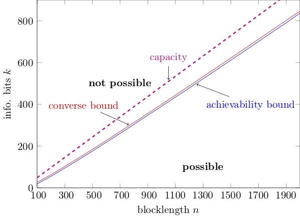
This is essentially the same figure I showed in part 2, but now I have put information bits rather rate on the y-axis. The figure illustrates achievability and converse bounds on $k^\star(n,\epsilon)$ as a function of $n$ for $\epsilon=10^{-4}$ and $\rho=0$ dB (here, $\rho$ is the SNR associated to the reception of our BPSK symbols).

I also plotted in magenta the curve $k^\star(n,\epsilon)=C n$ with $C$ standing for channel capacity, which comes from an asymptotic capacity analysis. Please note that this curve is just an approximation that is valid only in the asymptotic limit $n\rightarrow \infty$.

The figure tells us that all $(k,n)$ pairs that lie above the converse (red) curve are not feasible, whereas the $(k,n)$ pairs that lie below the blue (achievability) curve are feasible. We cannot say anything about the pairs between the two curves. This is a consequence of the fact that we cannot determine $k^*(n,\epsilon)$ exactly because, as discussed in the previous post, finding it involves an exhaustive search over a number of codes that grow double-exponentially in $n$ for a fixed rate. Luckily, our bounds are tight and the region of $(k,n)$ pairs we cannot characterize is small.

Note also how more accurate the classification enabled by FBL-IT is compared to the one based on capacity.

In the remainder of this post, I will explain how to evaluate the achievability (blue) curve shown in the figure. I’ll discuss the converse bound in the next post.

The random-coding union bound with parameter s

Achievability bounds in finite-blocklength information theory give us a lower bound on $k^\star(n,\epsilon)$, and, hence on $R^\star(k,n)$, or, equivalently, an upper bound on $\epsilon^*(k,n)$ for a given SNR value.

Many such bounds are available in the literature: some are based on threshold decoding, such as the dependence-testing bound. Some are based on hypothesis testing such as the $\kappa\beta$ and the $\beta\beta$ bounds. Here, I will review a variation of the random-coding union (RCU) bound ¹, called RCU bound with parameter $s$ (RCUs) ². This bound, which gives the achievability curve showed in blue in the plot, is appealing because

• it is tight both in the normal and in the error-exponent regimes (I will review what this mean in a later post)
• it is reasonably easy to evaluate numerically
• it lends itself to an easy generalization to arbitrary, mismatch decoding rules. This allows for its applications in many setups of practical relevance, including when one uses pilot symbols to estimate the channel in a fading environment, and nearest-neighbor detection based on the estimated CSI at the receiver.

Like most achievability bounds in information theory, the RCUs bound relies on random coding. What does this mean? The goal is, for fixed $k$ and $n$, to produce a code whose probability of error can be upper-bounded by a function of $k$ and $n$ that is reasonably easy to compute. The proof methodology is, however, not constructive in that it does not give us an actual code.

Indeed, rather than analyzing the performance of a given code, we analyze the average performance of a random ensemble of codes, whose codewords are drawn independently from a given input distribution. Then, we show that the average error probability, averaged over this ensemble is upper-bound by a suitable, easy-to-evaluate function of $k$ and $n$. Finally, we conclude that there must exist at least a code in the ensemble whose error probability is upper-bounded by that function.

I will state for future uses the RCUs bound in a more general setup than the bi-AWGN channel. Let us denote by $P_{Y^n | X^n}$ a general channel law that characterizes the input-output relation of blocks of $n$ symbols of a generic channel. For example, in the bi-AWGN case, we have

\[P_{Y^n | X^n}(y^n | x^n)=\prod_{j=1}^{n} P_{Y | X}(y_j | x_j)\]

where

\[P_{Y | X} (y |x)=\frac{1}{\sqrt{2\pi}}\exp\left(- \frac{(y-\sqrt{\rho}x)^2}{2} \right)\]

We are now ready to state the RCUs bound.

Fix an $s>0$ and an input distribution $P_{X^n}$. Then for every $k$ and $n$, there exists a $(k,n,\epsilon)$-code whose error probability is upper-bounded as

\(\epsilon \leq \mathbb{E}\left[ \exp\left[-\max\left\{0, \imath_s(X^n,Y^n)-(2^k-1) \right\} \right] \right].\)

Here, $(X^n,Y^n)$ is distributed as $P_{X^n}P_{Y^n | X^n}$ and $\imath_s(x^n,y^n)$ is the generalized information density, which is defined as \(\imath_s(x^n,y^n)=\log \frac{P^s_{Y^n | X^n} (y^n | x^n)}{\mathbb{E}\left[P^s_{Y^n | X^n}(y^n | \bar{X}^n)\right]}\) with $\bar{X}^n$ distributed as $P_{X^n}$ and independent of $X^n$.

I will next provide a proof for this bound. Implementation details, including a matlab script are given at the end of the post.

Let $M=2^k$ be the number of messages associated with the $k$ information bits. We assign to each message an $n$-dimensional codeword $C_j$, $j=1\dots,M$ generated independently from $P_{X^n}$. We shall analyze the average error probability under maximum-likelihood decoding, averaged with respect to all possible codewords generated in this way. The reader familiar with the derivation of Gallager’s random coding error exponent ³ will recognize most of the following steps. For a given realization $c_1,\dots,c_M$ of our random codebook, the error probability can be upper-bounded as

\[\epsilon(c_1,\dots,c_M) \leq \frac{1}{M} \sum_{j=1}^M \mathrm{Pr}\left[ \bigcup_{t=1, t\neq j}^M \left\{ P_{Y^n | X^{n}}(Y^n | c_t)\geq P_{Y^n | X^{n}}(Y^n | c_j) \right\} \right].\]

In words, under maximum-likelihood decoding, an error occurs whenever the transmitted codeword has a smaller likelihood than one of the other codewords. The inequality here comes from the fact that we assumed that all ties produce errors, which is pessimistic. We now average over all codebooks. Since all codewords are identically distributed, we can assume without loss of generality that the transmitted codeword is the first one. Hence,

\[\mathbb{E}\left[\epsilon(C_1,\dots,C_M)\right]\leq \mathrm{Pr}\left[ \bigcup_{t=2}^M \left\{ P_{Y^n | X^{n}}(Y^n | C_t)\geq P_{Y^n | X^{n}}(Y^n | C_1) \right\} \right].\]

The plan now is to replace the union by a sum by means of the union bound. However, to avoid the resulting bound to be too loose, we operate as follows. We first condition on $C_1$ and $Y^n$. Then we apply the union bound on $C_2,\dots,C_M$, and finally we average on $C_1$ and $Y^n$. These steps yield

\[\mathbb{E}\left[\epsilon(C_1,\dots,C_M)\right]\leq \mathbb{E}_{C_1,Y^n}\left[\min\left\{1,\sum_{t=2}^M\mathrm{Pr}\left[ P_{Y^n | X^{n}}(Y^n | C_t)\geq P_{Y^n | X^{n}}(Y^n | C_1) | C_1,Y^n \right]\right\}\right].\]

Here, the $\min$ tighten our results by ensuring that our upper bound on the probability term does not exceed $1$. Now, since all codewords $C_2,\dots,C_M$ are identically distributed, the $(M-1)$ probability terms are identical. Let us denote by $X^n$ the transmitted codeword and by $\bar{X^n}$ one of the other codewords:

\[P_{X^n,Y^n,\bar{X}^n}(x^n,y^n,\bar{x}^n)=P_{X^n}(x^n)P_{Y^n|X^n}(y^n|x^n)P_{X^n}(\bar{x}^n).\]

Using the observation above and the notation just introduced, we can rewrite our bound as

\[\epsilon \leq \mathbb{E}_{C_1,Y^n}\left[\min\left\{1, (M-1)\mathrm{Pr}\left[ P_{Y^n|X^n}(Y^n|\bar{X}^n)\geq P_{Y^n|X^n}(Y^n|X^n)| X^n,Y^n \right]\right\}\right]. \label{eq:RCU}\]

This is precisely the RCU bound proposed in ¹ .

Unfortunately, this bound is difficult to compute for the bi-AWGN channel. Indeed, no closed-form expression for the probability term in the bound is available. And a naïve Monte-Carlo approach to compute this term is unfeasible (although more sophisticated saddle-point approximation methods could be adopted instead). To see why, assume that $k=100$. Then, to compute the RCU bound, we would need to evaluate tail probabilities as small as $2^{-100}\approx 10^{-30}$.

One way to avoid this is to upper-bound the probability term using generalized Markov inequality. This inequality says that for every nonnegative random variable $T$ and for every nonnegative $s$,

\[\mathrm{Pr}[T>\gamma]\leq \frac{\mathbb{E}[T^s]}{\gamma^s}.\]

Applying this inequality to the probability term in the RCU bound, for fixed $X^n=x^n$ and $Y^n=y^n$, we obtain

\[\mathrm{Pr}\left[ P_{Y^n|X^n}(y^n|\bar{X}^n)\geq P_{Y^n|X^n}(y^n|x^n)\right]\leq \frac{\mathbb{E}\left[ P_{Y^n|X^n}^s(y^n|\bar{X}^n) \right]}{P^s_{Y^n|X^n}(y^n|x^n)}=e^{-\imath_s(x^n,y^n)}.\]

Substituting this inequality into the RCU bound \eqref{eq:RCU}, we obtain the desired RCUs bound after algebraic manipulations.

Evaluation of the RCUs for the bi-AWGN channel

To evaluate the RCUs bound for the bi-AWGN we just need to note that

\[\imath_s(x^n,y^n)= n\log 2 - \sum_{j=1}^n \log\left(1+e^{-2sx_jy_j\sqrt{\rho}}\right)\]

Few lines of matlab code suffice (author: Johan Östman, Chalmers).

function Pe = rcus_biawgn_fixed_s(R,n,rho,s,num_samples)
%this function computes rcus for given s
i_s = info_dens_biawgn(n,rho,s,num_samples);
Pe = mean( exp( - max(0, i_s - log(2^(n*R)-1) ) ));
end


function i_s = info_dens_biawgn(n,rho,s,num_samples)
S = [-sqrt(rho), sqrt(rho)]; %constellation
W = randn(num_samples, n); %create awgn noise
X = S(randi([1,2], num_samples, n)); %sample uniformly from constellation
Y = X+W; % add noise
i_s = sum(log(2) - (s/2)*(Y-X).^2 - log(exp(-(s/2)*(Y-S(1)).^2) + exp(-(s/2)*(Y-S(2)).^2)),2); %compute information density samples
end

---

Go to back to part 2 or move on to part 4

1. Y. Polyanskiy, H. V. Poor, and S. Verdú, “Channel coding rate in the finite blocklength regime,” IEEE Trans. Inf. Theory, vol. 56, no. 5, pp. 2307–2359, May 2010. ↩ ↩²

2. A. Martinez and A. Guillén i Fàbregas, “Saddlepoint approximation of random–coding bounds,” in Proc. Inf. Theory Applicat. Workshop (ITA), San Diego, CA, U.S.A., Feb. 2011. ↩

3. Section 5.6 of R. G. Gallager, Information Theory and Reliable Communication, New York, NY, U.S.A., 1968. ↩