Chapter 3 The binary-input AWGN channel
3.1 The tradeoff between transmission rate and packet error probability
We will start our tour through finite-blocklength information theory by analyzing one of the simplest, yet practically relevant, point-to-point communication channel: the discrete-time binary-input AWGN channel. The input-output relation of such a channel is \[\begin{equation} y_j=\sqrt{\rho}x_j + w_j, \quad j=1,\dots, n. \tag{3.1} \end{equation}\] Here, \(x_k\) is the channel input, which we assume to belong to the set \(\{-1,1\}\) whereas \(\{w_j\}\) is the discrete-time AWGN process. We assume it to be stationary memoryless and that each of its samples has zero mean and unit variance. Hence, \(\rho\) can be interpreted as the signal-to-noise ratio (SNR). Throughout, we shall assume that, to transmit an information message, i.e., a set of \(k\) information bits, we are allowed to use the bi-AWGN channel \(n\) times.
Note that \(n\) is closely related to the communication latency. Indeed, assume that to carry each binary symbol \(x_k\) we use a continuous-time signal of bandwidth \(W\) Hz. Then using the channel \(n\) times to transmit our message of \(k\) bits entails a delay of \(n/W\) seconds. The actual overall delay may be larger if we also include queuing, propagation, and decoding delays. But in a first approximation, we will neglect these additional sources of delay and take \(n\) as a proxy for latency. This is not a bad assumption for short-distance communications. In 4G for example, the smallest packet size has a duration of 0.5 milliseconds, whereas the propagation delay to cover a distance of 180 meters is just 30 microseconds.
So if we are interested in low latency, we should choose \(n\) as small as possible. But there is a tradeoff between latency and reliability. Indeed, it is intuitively clear that the larger the number of channel uses \(n\) we are allowed to occupy for the transmissions of our \(k\) bits is, the more reliable the transmission will be. Let us then denote by \(\epsilon\) the error probability. We are interested in the following question.
Fundamental question:
What is the smaller \(n\) for which the \(k\) information bits can be decoded correctly with probability \(1-\epsilon\) or larger?
Equivalently, we may try to find the largest number of bits \(k\) that we can transmit with reliability \(1-\epsilon\) or larger using the channel \(n\) times, or the smallest probability of error \(\epsilon\) that can be achieved for given \(k\) and \(n\).
What we will do next is to introduce some notation that will help us characterizing these quantities, and also illustrate why standard asymptotic information theory does not provide satisfactory answers.
How do we transmit the \(k\) information bits using \(n\) channel uses and how do we recover the \(k\) bits from the \(n\) received samples \(y^n=(y_1,\dots,y_n)\)? We use a channel code, i.e., an encoder that maps the \(k\) bits into the \(n\) channel uses, and a decoder that provides an estimate of the \(k\) information bits from \(y^n\).
Here is a more formal definition:
Definition 3.1 (Channel code) A \((k,n,\epsilon)\)-code for the bi-AWGN channel with a given SNR \(\rho\) consists of
- an encoder \(f:\{1,2,\dots, 2^k\}\mapsto \{-1,1\}^n\) that maps the information message \(\jmath \in \{1,2,\dots, 2^k\}\) into \(n\) BPSK symbols. We will refer to the set of all \(n\)-dimensional strings produced by the encoder as codebook. Furthermore, we will call each of the string a codeword and \(n\) the blocklength.
- A decoder \(g:\mathbb{R}^n\mapsto \{1,2,\dots, 2^k\}\) that maps the received sequence \(y^n \in \mathbb{R}^n\) into a message \(\widehat{\jmath}\in \{1,2,\dots, 2^k\}\), or, possibly, it declares an error. This decoder satisfies the error-probability constraint \(\mathbb{P}\bigl\{\widehat{\jmath}\neq \jmath\bigr\}\leq \epsilon\)
Note that \(\epsilon\) should be interpreted as a packet/frame error probability and not as a bit error probability. Indeed, a difference in a single bit between the binary representation of \(\jmath\) and \(\widehat{\jmath}\) causes an error, according to our definition.
In a nutshell, finite-blocklength information theory allows us to find, for a given SNR, the triplets \((k,n,\epsilon)\) for which a \((k,n,\epsilon)\)-code can be found and the triplets \((k,n,\epsilon)\) for which no code exists.
Note that doing so is not trivial, since an exhaustive search among all codes is hopeless. Indeed, even if we fix the decoding rule to, say, maximum likelihood, for a given choice of \(k\) and \(n\), one would in principle need to go through \(\binom{2^n}{2^k}\) codes. So for example, if we have \(k=5\) and \(n=10\), the number of codes is about \(5\times 10^{60}\). This means that even if we had a method to evaluate the error probability of a given code in \(1\) ms, it would still take \(2\times 10^{50}\) years to analyze all possible codes.
Before exploring how and in which sense a characterization of the triplets \((k,n,\epsilon)\) can be performed, let us first see what we can do by using the notion of channel capacity introduced by Shannon [3] in his groundbreaking paper, which started the field of information theory.
Let us denote by \(k^\star(n,\epsilon)\) the largest number of bits we can transmit using \(n\) channel uses with error probability not exceeding \(\epsilon\) and by \(R^\star(n,\epsilon)=(k^\star(n,\epsilon)/n)\log 2\) the corresponding maximum coding rate, measured in nats per channel use. Throughout this set of notes, it will be convenient to consistently measure all rates in nats per channel use rather than in bits per channel use, since it will simplify the theoretical derivations. This is why we multiplied the ratio \(k^\star(n,\epsilon)/n\) by \(\log 2\). In the numerical examples, we will however converts rates in the more familiar unit bit per channel use, by dividing \(R\) by \(\log 2\).
Also for a given rate \(R=(k/n) \log 2\), let us denote by \(\epsilon^\star(n,R)\) the smallest error probability achievable using \(n\) channel uses and a code of rate \(R\).
Since we cannot go through all possible codes, none of these quantities can be actually computed for the parameter values that are of interest in typical wireless communication scenarios. Actually, even for a given randomly chosen code, evaluating the error probability under the optimal maximum likelihood decoding is in general unfeasible. Shannon’s capacity provides an asymptotic characterization of these quantities.
Specifically, Shannon’s capacity \(C\) is the largest communication rate at which we can transfer information messages over a communication channel (in our case, the binary-input AWGN channel given in (3.1)) with arbitrarily small error probability for sufficiently large blocklength.
Mathematically,
\[\begin{equation} C=\lim_{\epsilon \to 0} \lim_{n\to \infty} R^\star(n,\epsilon). \end{equation}\]
Some remarks about this formula are in order:
One should in general worry about the existence of the limits in the definition of capacity that we have just provided. They do exist for the bi-AWGN channel under analysis here.
It is important to take the limits in this precise order. If we were to invert the order of the limits, we would get \(C=0\) for the bi-AWGN channel (3.1)—a not very insightful result.
For the channel in (3.1) (and for many other channels of interest in wireless communications), the first limit \(\epsilon\to 0\) is actually superfluous. We get the same result for every \(\epsilon\) in the interval \((0,1)\) as a consequence of the so-called strong converse theorem. We will show later in this set of notes why this is indeed the case and for which channels this property does not hold.
One way to explain the relation between capacity and finite-blocklength metrics is through the following figure, which artistically illustrates \(\epsilon^\star(n,R)\) as a function for \(R\) for various values of \(n\).
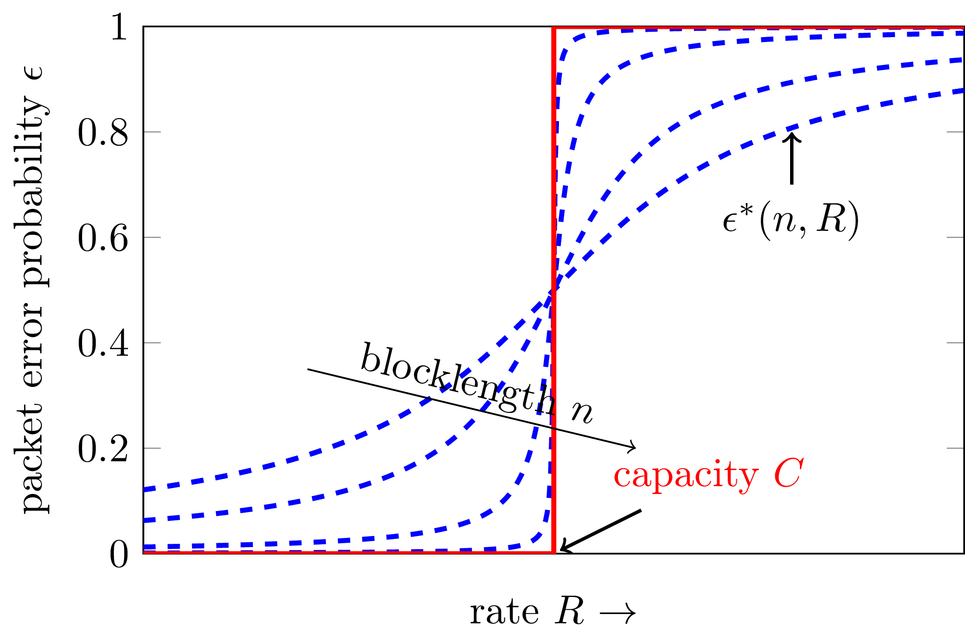
Figure 3.1: Error probability as a function of the rate
Although we do not know how to compute \(\epsilon^\star(n,R)\), Shannon was able to show that this function converges to a step function centered at \(C\) in the limit \(n\to\infty\). This means that when \(R<C\), one can achieve arbitrarily low \(\epsilon\) by choosing \(n\) sufficiently large. If however \(R>C\) the packet error probability goes to \(1\) as we increase \(n\).
We know from Shannon’s channel coding theorem that, for stationary memoryless channels like the binary input AWGN channel (3.1), the channel capacity \(C\) is
\[\begin{equation} C=\max_{P_X} I(X;Y) \tag{3.2} \end{equation}\]
where \(P_X\) denotes the probability distribution on the input \(X\) and \(I(X;Y)\) is the mutual information
\[\begin{equation} I(X;Y)= \mathbb{E}\left[\log\frac{P_{Y|X}(Y|X)}{P_Y(Y)}\right]. \tag{3.3} \end{equation}\]
Here, the expectation is with respect to the joint distribution of \((X,Y)\). Furthermore, \(P_{Y|X}\) denotes the channel law
\[\begin{equation} P_{Y | X} (y |x)=\frac{1}{\sqrt{2\pi}}\exp\left(- \frac{(y-\sqrt{\rho}x)^2}{2} \right) \tag{3.4} \end{equation}\]
and \(P_Y\) is the distribution on the channel output \(Y\) induced by \(P_X\) through \(P_{Y| X}\). Specifically, \(P_Y(y)=\mathbb{E}\left[P_{Y|X}(y|\bar{X})\right]\) where \(\bar{X}\sim P_X\) and independent of \(X\).
A remark on notation is in order. It will be convenient from now on to distinguish between deterministic and random quantities. We will use uppercase letters such as \(X\) to denote random quantities, and lowercase letters such as \(x\) to denote their realizations.
It will also be convenient to give a name to the log-likelihood ratio in the argument of the expectation that defines mutual information in (3.3). It is usually called information density and denoted by \(\imath(x,y)\). Hence, \(I(X;Y)=\mathbb{E}[\imath(X,Y)]\).
For the bi-AWGN channel, one can show that the uniform distribution over \(\{-1,1\}\) achieves the maximum in (3.2). The induced output distribution \(P_Y\) is a Gaussian mixture \[P_Y= \frac{1}{2}\mathcal{N}(-\sqrt{\rho},1)+\frac{1}{2}\mathcal{N}(\sqrt{\rho},1)\] and the information density can be readily computed as \[\begin{equation} \imath(x,y) = \log 2 - \log\left(1+ \exp(-2xy\sqrt{\rho})\right) \tag{3.5} \end{equation}\]
Finally, the channel capacity \(C\) (measured in nats per channel use) is given by
\[\begin{equation} C=\frac{1}{\sqrt{2\pi}}\int e^{-z^2/2} \Bigl(\log 2-\log\bigl(1+e^{-2\rho-2z\sqrt{\rho}}\bigr) \Bigr)\, \mathrm{d}z. \tag{3.6} \end{equation}\]
Computing capacity takes only few lines of matlab code
f = @(z) exp(-z.^2/2)/sqrt(2*pi) .* (log2(2) - log2(1+exp(-2*rho-2*sqrt(rho)*z)));
Zmin = -9; Zmax = 9;
C = quadl(f, Zmin, Zmax);
This code is part of the routine biawgn_stats.m available as part of the SPECTRE toolbox. We will talk about this toolbox in later chapters; nevertheless, it may be good to have a look at it already now.
To summarize, the capacity of the bi-AWGN channel is relatively easy to compute, but gives us only the following asymptotic answer to the question about which triplets \((k,n,\epsilon)\) are achievable:
Asymptotic wisdom: All triplets \((nR/\log 2,n,\epsilon)\) are achievable for sufficiently large \(n\), provided that \(R<C\).
Although asymptotic, the characterization of the achievable triplets provided by Shannon’s capacity has turned out to be very important! Not only it provides a benchmark against which to compare the performance of actual codes. It also provides a useful abstraction of the physical layer (especially when capacity is known in closed form), which can be used for the design of higher-layer protocols, such as resource allocation and user scheduling algorithms.
Unfortunately, the asymptotic answer provided by Shannon’s capacity turns out to be loose when the blocklength \(n\) is small. As we shall see, finite-blocklength information theory will give us a much more precise characterization.
Let us go back to the tradeoff between \(\epsilon\) and \(R\) depicted artistically in Fig. 3.1. In Fig. 3.2 below, we show how finite-blocklength information theory can be used to provide a very accurate quantitative characterization of this trade-off for a fixed blocklength \(n\).
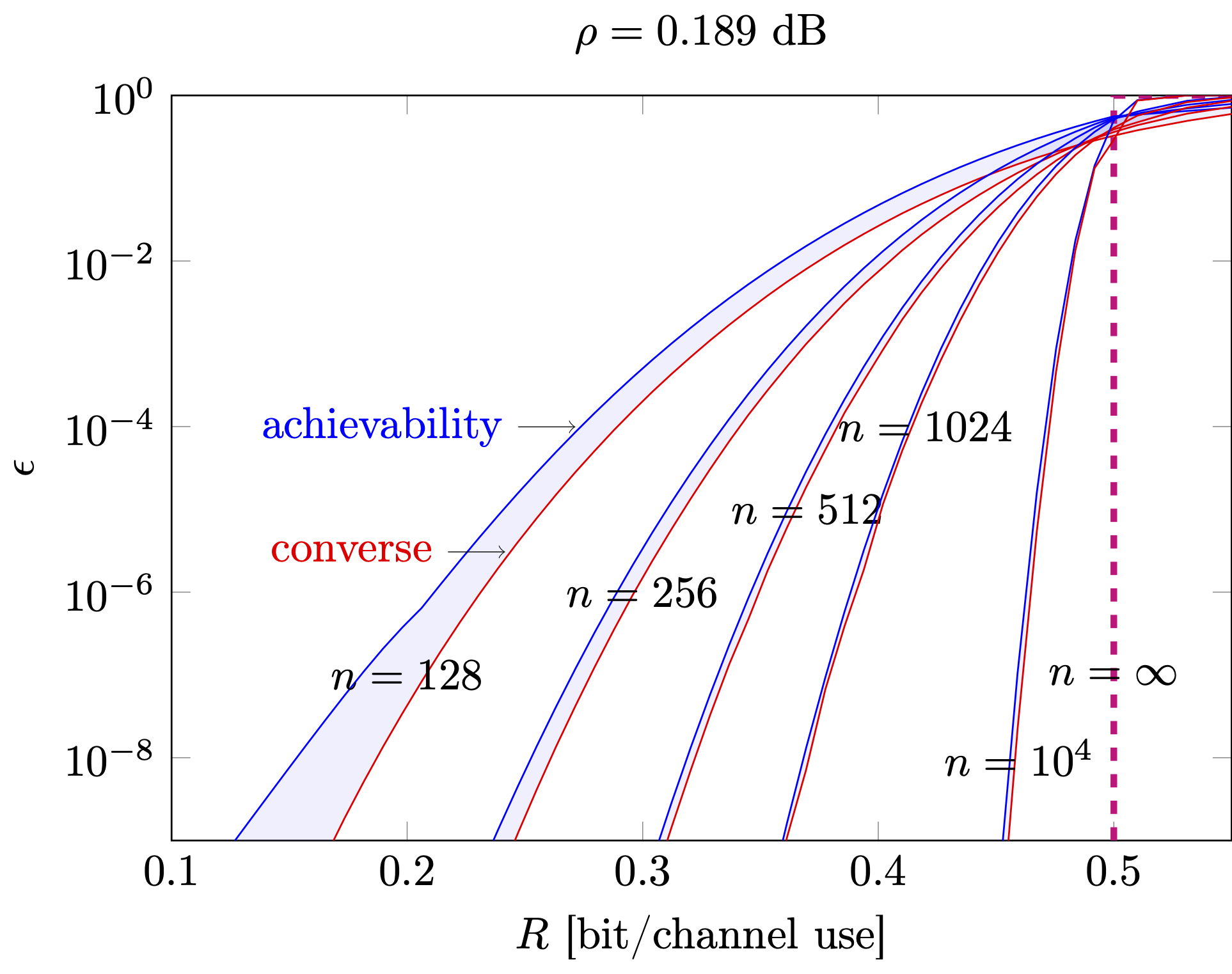
Figure 3.2: Finite-blocklength upper and lower bounds on \(\epsilon^*(n,R)\) as a function of the rate \(R\) measured in bits per channel use for different values of the blocklength \(n\)
In the figure we have set \(\rho=0.189\) dB. For this value of SNR, the Shannon capacity is equal to \(0.5\) bits per channel use. As shown by the dashed vertical red line in the figure, this implies that for all rates below \(0.5\) bits per channel use an arbitrary low error probability can be achieved by letting the blocklength \(n\to\infty\). The other curves in the figure illustrate upper (achievability) bounds in blue and lower (converse) bounds on the error probability \(\epsilon^*(n,R)\) for different values of the blocklength \(n\). The converse bounds give us an impossibility result: for a given blocklength, no code with parameters \(\{R,\epsilon(R,n)\}\) that lie below the red curve can be found. The achievability result instead demonstrates the existence of codes with parameters \(\{R,\epsilon(R,n)\}\) above the blue curve (although, it does not indicate how to construct them explicitly). Between the two curves lies a (small) region for which we cannot prove or disprove the existence of a code.
Here is how we can use this figure for system design. If, for example, we want codes operating at an error probability of \(\epsilon=10^{-8}\), Fig. 3.2 tells us that for a blocklength of \(128\) channel uses, we should use a code of rate below \(0.19\) bits/channel use. However, if we can afford a blocklength of \(512\) channel uses, codes with rate as large as \(0.31\) bits per channel uses can be used. Both values are significantly smaller than the \(0.5\) bits per channel use promised by the Shannon capacity.
3.2 An achievability bound
3.2.1 The random-coding union bound with parameter s
As already mentioned, achievability bounds in finite-blocklength information theory give us an upper bound on \(\epsilon^*(k,n)\), or equivalently, a lower bound on \(k^\star(n,\epsilon)\), and, hence on \(R^\star(k,n)\) for a given SNR value.
Many such bounds are available in the literature: some are based on threshold decoding, such as the dependence-testing bound [1]. Some are based on hypothesis testing such as the \(\kappa\beta\) bound [1] and the \(\beta\beta\) bound [4]. Here, we will review a variation of the random-coding union (RCU) bound in [1] introduced in [5], which is commonly referred to as RCU bound with parameter \(s\) (RCUs).
This bound is appealing because
- it is tight for a large range of error-probability values
- it is reasonably easy to evaluate numerically
- it lends itself to an easy generalization to arbitrary, mismatch decoding rules. This is important, because it enables its applications in many setups of practical relevance, including when one uses pilot symbols to estimate the channel in a fading environment, and nearest-neighbor detection based on the estimated CSI at the receiver.
Like most achievability bounds in information theory, the RCUs bound relies on random coding, a technique introduced by Shannon [3] to establish achievability results. The idea is as follows: rather than analyzing the performance of a given code, one analyzes the average performance of a random ensemble of codes, whose codewords are drawn independently from a given distribution. Then, one shows that the average error probability, averaged over this ensemble is upper-bound by a suitable, easy-to-evaluate function of \(k\) and \(n\). Finally, one concludes that there must exist at least a code in the ensemble whose error probability is upper-bounded by that function.
We will state for future uses the RCUs bound in a more general setup than the bi-AWGN channel. Specifically, let us denote by \(P_{Y^n | X^n}\) a general channel law that describes in probabilistic terms the input-output relation corresponding to the transmission of a block of \(n\) symbols over a generic channel. For example, in the bi-AWGN case, we have
\[P_{Y^n | X^n}(y^n | x^n)=\prod_{j=1}^{n} P_{Y | X}(y_j | x_j)\]
where \(P_{Y | X}(y |x)\) was given in (3.4).
We are now ready to state the RCUs bound.
Note that the generalized information density in (3.8) is closely related to the information density in (3.5) and the two quantities coincide for the case \(s=n=1\). We will next prove (3.7). Implementation details for the case of the bi-AWGN channel, including a matlab script, are given at the end of this section.
Proof. Let \(M=2^k\) be the number of messages associated with the \(k\) information bits. We assign to each message an \(n\)-dimensional codeword \(C_j\), \(j=1,\dots,M\) generated independently from an \(n\)-dimensional distribution \(P_{X^n}\). We shall analyze the average error probability under maximum-likelihood decoding, averaged with respect to all possible codewords generated in this way. The reader familiar with the derivation of Gallager random coding error exponent [6] will recognize most of the following steps. For a given realization \(c_1,\dots,c_M\) of our random codebook, the error probability can be upper-bounded as
\[\epsilon(c_1,\dots,c_M) \leq \frac{1}{M} \sum_{j=1}^M \mathbb{P}\left[ \bigcup_{t=1, t\neq j}^M \left\{ P_{Y^n | X^{n}}(Y^n | c_t)\geq P_{Y^n | X^{n}}(Y^n | c_j) \right\} \right]. \]
In words, under maximum-likelihood decoding, an error occurs whenever the transmitted codeword has a smaller likelihood than one of the other codewords. The inequality here comes from the fact that we assumed that all ties produce errors, which is pessimistic. We now average over all codebooks. Since all codewords are identically distributed, we can assume without loss of generality that the transmitted codeword is the first one. Hence,
\[\mathbb{E}\left[\epsilon(C_1,\dots,C_M)\right]\leq \mathbb{P}\left[ \bigcup_{t=2}^M \left\{ P_{Y^n | X^{n}}(Y^n | C_t)\geq P_{Y^n | X^{n}}(Y^n | C_1) \right\} \right]. \]
The plan now is to replace the probability of the union of events by a sum of probabilities of individual events by means of the union bound. However, to make sure that the resulting bound is not too loose, we operate as follows. We first condition on \(C_1\) and \(Y^n\). Then, we apply the union bound with respect to \(C_2,\dots,C_M\), and finally we average over \(C_1\) and \(Y^n\). These steps yield
\[\mathbb{E}\left[\epsilon(C_1,\dots,C_M)\right]\leq \mathbb{E}_{C_1,Y^n}\left[\min\left\{1,\sum_{t=2}^M\mathbb{P}\left[ P_{Y^n | X^{n}}(Y^n | C_t)\geq P_{Y^n | X^{n}}(Y^n | C_1) | C_1,Y^n \right]\right\}\right]. \]
Here, the \(\min\) tightens our results by ensuring that our upper bound on the probability term does not exceed \(1\). Now, since all codewords \(C_2,\dots,C_M\) are identically distributed, the \((M-1)\) probability terms are identical. Let us denote by \(X^n\) the transmitted codeword and by \(\bar{X^n}\) one of the other codewords. Using the observation above and the notation just introduced, we can rewrite our bound as
\[\begin{equation} \epsilon \leq \mathbb{E}_{X^n,Y^n}\left[\min\left\{1, (M-1)\mathbb{P}\left[ P_{Y^n|X^n}(Y^n|\bar{X}^n)\geq P_{Y^n|X^n}(Y^n|X^n)| X^n,Y^n \right]\right\}\right]. \tag{3.9} \end{equation}\] This is precisely the RCU bound proposed in [1] .
Unfortunately, this bound is difficult to compute for the bi-AWGN channel. Indeed, no closed-form expression for the probability term in the bound is available. And a naïve Monte-Carlo approach to compute this term is unfeasible (although more sophisticated saddle-point approximation methods could be adopted instead [7]—we will review them in a later chapter). To see why, assume that \(k=100\) so that \(M=2^k=2^{100}\). Then, to compute the RCU bound, we would need to evaluate numerically tail probabilities as small as \(2^{-100}\approx 10^{-30}\).
One way to avoid this is to upper-bound the probability term using the generalized Markov inequality. This inequality states that for every nonnegative random variable \(T\) and for every positive \(s\),
\[ \mathbb{P}[T>\gamma]\leq \frac{\mathbb{E}[T^s]}{\gamma^s}.\]
Applying this inequality to the probability term in the RCU bound, for fixed \(X^n=x^n\) and \(Y^n=y^n\), we obtain
\[\begin{equation} \mathbb{P}\left[ P_{Y^n|X^n}(y^n|\bar{X}^n)\geq P_{Y^n|X^n}(y^n|x^n)\right]\leq \frac{\mathbb{E}\left[ P_{Y^n|X^n}^s(y^n|\bar{X}^n) \right]}{P^s_{Y^n|X^n}(y^n|x^n)}=e^{-\imath_s(x^n;y^n)}. \tag{3.10} \end{equation}\]
Substituting this inequality into the RCU bound (3.9), we obtain the desired RCUs bound after algebraic manipulations.3.2.2 Evaluation of the RCUs for the bi-AWGN channel
To evaluate the RCUs bound for the bi-AWGN we just need to note that \[\begin{equation} \imath_s(x^n,y^n)= n\log 2 - \sum_{j=1}^n \log\left(1+e^{-2sx_jy_j\sqrt{\rho}}\right) \tag{3.11} \end{equation}\]
Few lines of matlab code suffice (author: Johan Östman, Chalmers).
function Pe = rcus_biawgn_fixed_s(R,n,rho,s,num_samples)
%this function computes rcus for given s
i_s = info_dens_biawgn(n,rho,s,num_samples);
Pe = mean( exp( - max(0, i_s - log(2^(n*R)-1) ) ));
end


function i_s = info_dens_biawgn(n,rho,s,num_samples)
S = [-sqrt(rho), sqrt(rho)]; %constellation
W = randn(num_samples, n); %create awgn noise
X = S(randi([1,2], num_samples, n)); %sample uniformly from constellation
Y = X+W; % add noise
i_s = sum(log(2) - (s/2)*(Y-X).^2 - log(exp(-(s/2)*(Y-S(1)).^2) + exp(-(s/2)*(Y-S(2)).^2)),2); %compute information density samples
end
3.3 A converse bound
Converse bounds in information theory express an impossibility condition. In our case, a converse result says that no \((k,n,\epsilon)\)-code can be found for which the triplets \((k,n,\epsilon)\) violate a certain relation. Converse bounds give a lower bound on the error probability \(\epsilon^\star(k,n)\), or equivalently, an upper bound on \(k^\star(n,\epsilon)\) and, hence, on \(R^\star(k,n)\).
We will review in this section a very general technique to obtain converse bounds in finite-blocklength information theory, which relies on the so-called metaconverse theorem [1].
3.3.1 Binary hypothesis testing
Before introducing the metaconverse theorem, we need to review some basic concepts in binary hypothesis testing.
Binary hypothesis testing deals with the following problem (see figure below). We observe a vector \(X^n\) which may have been generated according to a distribution \(P_{X^n}\) or according to an alternative distribution \(Q_{X^n}\). Our task is to decide which of the two distributions generated \(X^n\).
To do so, we design a test \(Z\) whose input is the vector \(X^n\) and whose output is a binary value \(\{0,1\}\). We use the convention that \(0\) indicates that the test chooses \(P_{X^n}\) and \(1\) indicates that the test chooses \(Q_{X^n}\).
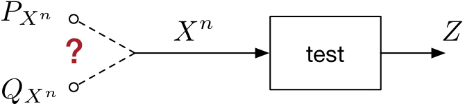
Figure 3.3: Binary hypothesis testing
We can think of the test \(Z\) as a binary partition of the set of the vectors \(X^n\).
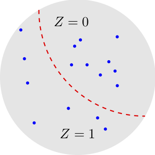
Figure 3.4: Binary hypothesis testing as a binary partition
Actually, we will need the more general notion of randomized test, in which the test is a conditional distribution \(P_{Z |X^n}\). Coarsely speaking, for some values of \(X^n\), we may flip a coin to decide whether \(Z=0\) or \(Z=1\). It turns out that this randomization is needed at the boundary between the two regions.
We are interested in the test that minimizes the probability of misclassification when \(X^n\) is generated according to \(Q_{X^n}\) given that the probability of correct classification under \(P_{X^n}\) is above a given target. Mathematically, we define the probability of misclassification under \(Q_{X^n}\) as
\[Q_{X^n}[Z=0]=\sum_{x^n}Q_{X^n}(x^n)P_{Z | X^n}(0 | x^n). \]
To parse this expression, recall that \(Z=0\) means that the test chooses \(P_{X^n}\), which is the wrong distribution in this case. Here, we assumed for simplicity that \(X^n\) is a discrete random variable. For the continuous case, one needs to replace the sum with an integral. The probability of correct classification under \(P_{X^n}\) is similarly given by
\[P_{X^n}[Z=0]=\sum_{x^n}P_{X^n}(x^n)P_{Z | X^n}(0 | x^n).\]
We let \(\beta_{\alpha}(P_{X^n},Q_{X^n})\) be the Neyman-Pearson beta function, which denotes the smallest possible misclassification probability under \(Q_{X^n}\) when the probability of correct classification under \(P_{X^n}\) is at least \(\alpha\):
\[\beta_{\alpha}(P_{X^n},Q_{X^n})=\inf_{P_{Z| X^n}: P_{X^n}[Z=0]\geq \alpha} Q_{X^n}[Z=0].\]
It follows from the Neyman-Pearson lemma (see e.g., p. 144 of the following lecture notes) that \(\beta_{\alpha}(P_{X^n},Q_{X^n})\) is achieved by the test that computes the log-likelihood ratio \(\log \frac{P_{X^n}(x^n)}{Q_{X^n}(x^n)}\) and sets \(Z=0\) if the log-likelihood is above a threshold \(\gamma\); it sets \(Z=1\) otherwise. Here, \(\gamma\) is chosen so that
\[P_{X^n}\left[\log \frac{P_{X^n}(x^n)}{Q_{X^n}(x^n)} \geq \gamma \right]=\alpha.\]
Note that to satisfy this equality, one needs in general to use a randomized test that flips a suitably biased coin whenever \(\log \frac{P_{X^n}(x^n)}{Q_{X^n}(x^n)} = \gamma\).
One may wonder at this point what binary hypothesis testing has to do with channel coding. Surely, decoding involves a hypothesis test. The test, however, is not binary but \(M\)-ary, since it involves \(M=2^k\) codewords. We will see later on in this section why such a binary hypothesis test emerges naturally. We provide for the moment the following intuition.
Consider the binary hypothesis testing problem in which one has to decide whether the pair \((X^n, Y^n)\) comes from \(P_{X^n,Y^n}\) or from \(P_{X^n}P_{Y^n}\). Assume that all distributions are product distributions, i.e.,
\[ P_{X^n,Y^n}(x^n,y^n)=\prod_{j=1}^n P_{X,Y}(x_j,y_j)\]
then Stein’s lemma (see page 147 of [8]) implies that for all \(\alpha \in (0,1)\)
\[ \beta_{\alpha}(P_{X^n,Y^n},P_{X^n}P_{Y^n}) = e^{-n\bigl[I(X;Y) + o(1)\bigr]},\quad n\to\infty.\]
Here, \(o(1)\) stands for terms that go to zero when \(n\rightarrow \infty\).
In words \(\beta_{\alpha}(P_{X^n,Y^n},P_{X^n}P_{Y^n})\) decays exponentially fast in \(n\), with an exponent given by the mutual information \(I(X;Y)\). So if mutual information is useful in characterizing the performance of a communication system in the asymptotic limit \(n\to\infty\), it makes sense that the Neyman-Pearson \(\beta\) function is useful to describe performance at finite blocklength.
3.3.2 The metaconverse bound
We are now ready to state our converse bound, which we shall refer to as metaconverse theorem although this term is used in [1] for a slightly more general result. As for the RCUs bound in Theorem 3.1, we will first state and prove the bound for a general channel \(P_{Y^n|X^n}\). Then, we will particularize it to the bi-AWGN channel.
Theorem 3.2 (metaconverse) Fix an arbitrary \(Q_{Y^n}\). Every \((k,n,\epsilon)\)–code must satisfy
\[\begin{equation} 2^k\leq \sup_{P_{X^n}}\frac{1}{\beta_{1-\epsilon}(P_{X^n}P_{Y^n|X^n},P_{X^n}Q_{Y^n})}. \tag{3.12} \end{equation}\]Proof. Fix a \((k,n,\epsilon)\)–code and let \(P_{X^n}\) be the distribution induced by the encoder on the transmitted symbol vector \(X^n\). We now use the code to perform a binary-hypothesis test between \(P_{X^n}P_{Y^n |X^n}\) and \(P_{X^n}Q_{Y^n}\). Specifically, for a given pair \((X^n,Y^n)\) we determine the corresponding transmitted message \(W\) by inverting the encoder given its output \(X^n\). We also find the decoded message \(\hat{W}\) by applying the decoder to \(Y^n\). If \(W=\hat{W}\), we set \(Z=0\) and choose \(P_{X^n}P_{Y^n |X^n}\). Otherwise, we set \(Z=1\) and choose \(P_{X^n}Q_{Y^n}\).
Since the given code has an error probability no larger than \(\epsilon\) when used on the channel \(P_{Y^n |X^n}\), we conclude that
\[P_{X^n}P_{Y^n |X^n}[Z=0]\geq 1-\epsilon. \]
The misclassification probability under the alternative hypothesis \(P_{X^n}Q_{Y^n}\) is the probability that the decoder produces a correct message when the channel output \(Y^n\) is distributed according to \(Q_{Y^n}\), and, hence, is independent of the channel input \(X^n\). This probability, which is equal to \(1/2^k\) is no larger than the misclassification probability of the optimal test \(\beta_{1-\epsilon}(P_{X^n}P_{Y^n|X^n},P_{X^n}Q_{Y^n})\). Mathematically,
\[\beta_{1-\epsilon}(P_{X^n}P_{Y^n|X^n},P_{X^n}Q_{Y^n})\leq P_{X^n}Q_{Y^n}[Z=0]=\frac{1}{2^k}. \]
Hence, for the chosen \((k,n,\epsilon)\)–code, we have
\[\begin{equation} 2^k\leq \frac{1}{\beta_{1-\epsilon}(P_{X^n}P_{Y^n|X^n},P_{X^n}Q_{Y^n})}. \tag{3.13} \end{equation}\]
We finally maximize over \(P_{X^n}\) to obtain a bound that holds for all \((k,n,\epsilon)\) codes. This concludes the proof.How tight is this bound? It turns out that, for a given code with maximum-likelihood decoder, the bound given in (3.13) is tight provided that the auxiliary distribution \(Q_{Y^n}\) is chosen in an optimal way.
Specifically, set \(Q^\star_{Y^n}(y^n)=\frac{1}{\mu}\max_{\bar{x}^n}P_{Y^n|X^n}(y^n|\bar{x}^n)\) where \(\mu\) is a normalization constant chosen so that \(Q^\star_{Y^n}\) integrates to \(1\). Note now that, for a given transmitted codeword \(x^n\), the optimum ML decoder finds the correct codeword (under the simplifying assumption of no ties) provided that
\[P_{Y^n|X^n}(y^n|x^n)\geq \max_{\bar{x}^n}P_{Y^n|X^n}(y^n|\bar{x}^n).\]
This is the same as requiring that
\[ \log\frac{P_{Y^n|X^n}(y^n|x^n)}{Q^\star_{Y^n}(y^n)}\geq \log \mu. \]
Furthermore, observe that, since the code has probability of error \(\epsilon\) under ML decoding, the following must hold:
\[P_{X^n}P_{Y^n|X^n}\left[\log\frac{P_{Y^n|X^n}(y^n|x^n)}{Q^\star_{Y^n}(y^n)}\geq \log \mu\right]=1-\epsilon \]
Hence,
\[\beta_{1-\epsilon}(P_{X^n}P_{Y^n|X^n},P_{X^n}Q_{Y^n})=P_{X^n}Q_{Y^n}\left[\log\frac{P_{Y^n|X^n}(y^n|x^n)}{Q^\star_{Y^n}(y^n)}\geq \log \mu\right]=\frac{1}{2^k}.\]
3.3.3 Evaluation of the metaconverse bound for the bi-AWGN channel
At first glance, evaluating the metaconverse bound seems hard because of the maximization over \(P_{X^n}\) in (3.12). It turns out that, for some channels like the bi-AWGN channel under consideration here, this maximization can be avoided altogether by choosing the auxiliary distribution \(Q_{Y^n}\) in a suitable way.
Specifically, let \[P_Y= \frac{1}{2}\mathcal{N}(-\sqrt{\rho},1)+\frac{1}{2}\mathcal{N}(\sqrt{\rho},1)\] be the capacity achieving output distribution of our binary-input AWGN channel, i.e., the output distribution induced by the capacity-achieving input distribution (which, as already mentioned, is uniform).
We choose \(Q_{Y^n}\) so that the resulting vector \(Y^n\) has independent entries, all distributed according to \(P_Y\). The key observation now is that because of symmetry, for every binary channel input \(x^n\) \[\begin{equation} \beta_{1-\epsilon}(P_{Y^n | X^n=x^n}, Q_{Y^n} )= \beta_{1-\epsilon}(P_{Y^n | X^n=\bar{x}^n}, Q_{Y^n} ) \tag{3.14} \end{equation}\]
where \(\bar{x}^n\) is the all-one vector. One can then show (see Lemma 29 in [1]) that when (3.14) holds, then
\[\beta_{1-\epsilon}(P_{X^n}P_{Y^n|X^n},P_{X^n}Q_{Y^n})= \beta_{1-\epsilon}(P_{Y^n | X^n=\bar{x}^n}, Q_{Y^n} )\]
Note that the right-hand side of this equality does not depend on \(P_{X^n}\). Hence, for this (generally suboptimal) choice of \(Q_{Y^n}\), the metaconverse bound simplifies to
\[2^k\leq \frac{1}{ \beta_{1-\epsilon}(P_{Y^n | X^n=\bar{x}^n}, Q_{Y^n} )}.\]
Equivalently, \[\begin{equation} R \leq -\frac{1}{n}\log \biggl( \beta_{1-\epsilon}(P_{Y^n | X^n=\bar{x}^n}, Q_{Y^n} ) \biggr). \tag{3.15} \end{equation}\]
Note that the rate here is measured, as usual, in nats per channel use.
Evaluating the beta function directly through the Neyman-Pearson lemma is challenging, because the corresponding tail probabilities are not known in closed form, and one of them needs to evaluated with very high accuracy (we encountered the same problem when we discussed the evaluation of the RCU bound in Theorem 3.1). As we shall discuss later, one can use the saddlepoint methods to approximate these tail probabilities accurately [7].
A simpler approach is to further relax the bound using the following inequality on the \(\beta\) function (see p. 143 of [8]): \[\begin{equation} \beta_{1-\epsilon}(P_{Y^n| X^n=\bar{x}^n},Q_{Y^n}) \geq \sup_{\gamma > 0} \left\{e^{-\gamma}\left(1-\epsilon- P_{Y^n | X^n=\bar{x}^n}\left[\log \frac{P_{Y^n| X^n}(Y^n|\bar{x}^n)}{Q_{Y^n}(Y^n)}\geq \gamma\right]\right)\right\}. \tag{3.16} \end{equation}\]
The resulting bound, which is a generalized version of Verdú-Han converse bound [9] can be evaluated efficiently. It is given below: let \(\imath(x,y)\) be the information density defined in (3.5). It then follows from (3.16) and from our choice of the auxiliary distribution that
\[\begin{equation} R \leq \inf_{\gamma >0} \frac{1}{n}\biggl\{ \gamma - \log\biggl( (1-\epsilon) - P_{Y^n | X^n=\bar{x}^n}\biggl[ \sum_{k=1}^n \imath(x_k,y_k)\geq \gamma \biggr] \biggr) \biggr\}. \tag{3.17} \end{equation}\]
Here is a simple matlab implementation of this bound.
function rate=vh_metaconverse_rate(snr,n,epsilon,precision)
  idvec=compute_samples(snr,n,precision);
  idvec=sort(idvec);
  ratevec=zeros(length(idvec),1);
  for i=1:1:precision,
    prob=sum(idvec<idvec(i))/precision;
    ratevec(i)=idvec(i)-log(max(prob-epsilon,0));
  end
  rate=min(ratevec)/(n*log(2));
end


function id=compute_samples(snr,n,precision)
  normrv=randn(n,precision)*sqrt(snr)+snr;
  idvec=log(2)-log(1+exp(-2.*normrv));
  id=sum(idvec);
end
3.4 A numerical example
In Figure 3.5 below we depict the upper and lower bound on \(\epsilon^*(n,R)\) resulting by using the RCUs bound (3.7) (optimized over the parameter \(s\)) and the Verdú-Han relaxation of the metaconverse bound (3.17).
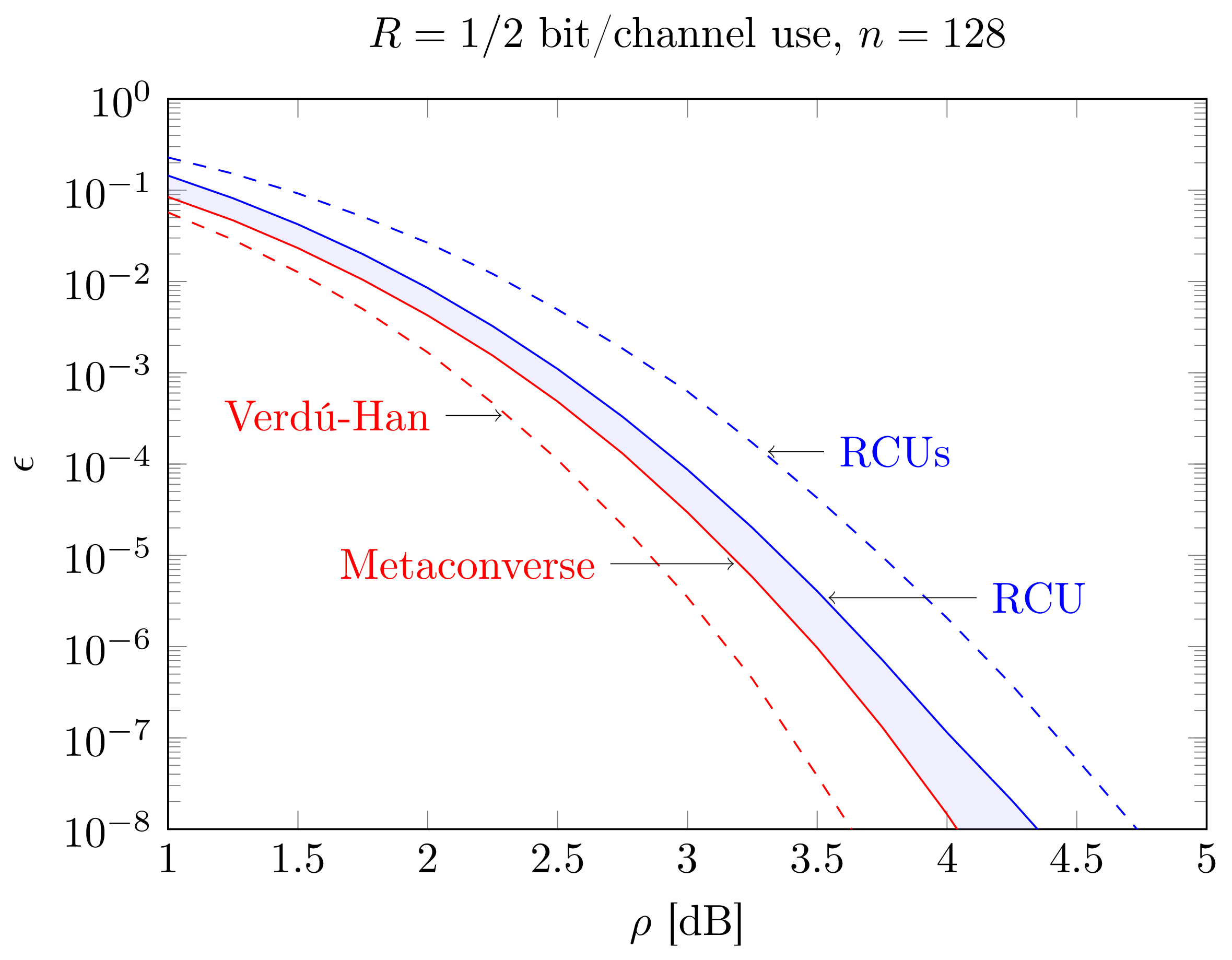
Figure 3.5: Finite-blocklength upper and lower bounds on \(\epsilon^*(n,R)\) as a function of the SNR (dB) for \(R=1/2\) bit/channel use and \(n=128\)
We assume that \(R=0.5\) bit/channel use and \(n=128\).
The figure shows the two bounds on the error probability as a function of the SNR \(\rho\).
As shown in the figure the two bounds we have just introduced are not the tightest available.
From an achievability bound perspective, one can tighten the RCUs bound by using instead the RCU bound (3.9) directly.
Since this bound is difficult to evaluate numerically for low error probabilities, the use of the saddlepoint approximation, which we shall introduce in a later chapter, is indispensable.
Also one can improve on the Verdú-Han relaxation of the metaconverse, by plotting the metaconverse directly (again with the help of a saddlepoint approximation) and by optimizing the chosen auxiliary distribution.
Specifically, the bound in the figure is obtained by considering as auxiliary distribution the so-called error-exponent achieving output distribution.
We will discuss this bound in a later chapter.
3.5 The normal approximation
Both the RCUs bound in Theorem 3.1 and the metaconverse bound in Theorem 3.2 are not in closed form and involve the numerical evaluation of \(n\)-dimensional integrals, which can be performed, for example, by means of Monte-Carlo simulations.
In this section, we will perform an asymptotic expansion of both bounds, which reveals that, when suitably optimized, the bounds are asymptotically tight. More precisely, the bounds allow one to characterize the first two terms of the asymptotic expansion of the maximum coding rate \(R^*(n,\epsilon)\) achievable on the bi-AWGN channel (3.1) for a fixed \(\epsilon\), as \(n\to\infty\). As we shall see, this expansion relies on the central limit theorem, and yields an approximation (obtained by neglecting the error terms in the expansion), which is usually referred to as normal approximation.
The key observation is that, for a suitable choice of the input distribution in Theorem 3.1 and of the output distribution in Theorem 3.2, both RCUs and metaconverse bounds turn out to involve the computation of the tail distribution of a sum of independent random variables. We have already seen that this is the case for the Verdú-Han relaxation (3.17) of the metaconverse.
We next demonstrate that this is also true for the RCUs bound in Theorem 3.1. To do so, we start by noting that, as we have already demonstrated in (3.11), for our choice of the input distribution, the generalized information density can be expressed as
\[ \imath_s(x^n,y^n)= \sum_{j=1}^n \imath_s(x_j,y_j) \] where \[\begin{equation} \imath_s(x_j,y_j)= \log 2 - \log(1+e^{-2s x_j y_j \sqrt{\rho}}). \tag{3.18} \end{equation}\] Let now \(U\) be a uniform random variable on \([0,1]\). We shall use that for every nonnegative random variable \(Z\), we have that \(\mathbb{E}[\min\{1,Z\}]= \mathbb{P}[Z\geq U]\) Using this result in (3.7), we obtain after some algebraic manipulations
\[\begin{align} \mathbb{E}\left[ \exp\left[-\max\left\{0, \imath_s(X^n,Y^n)-\log(2^k-1) \right\} \right] \right]\\ =\mathbb{P}\left[\sum_{j=1}^n \imath_s(X_j,Y_j) + \log U \leq \log(2^k-1)\right]. \tag{3.19} \end{align}\] This shows that the RCUs bound can indeed be written as the tail probability of a sum of independent random variables.
3.5.1 A normal approximation for the bi-AWGN channel
Before we state the normal approximation, we need to introduce some notation. Recall the information density we introduced in (3.5). As we have already noticed, the generalized information density \(\imath_s(x_j,y_j)\) in (3.18) coincides with the information density when \(s=1\), i.e., \[\imath_1(x_j,y_j)=\imath(x_j,y_j). \] Note also that the random variables \(\imath(X_j,Y_j)\) are independent and identically distributed. Furthermore, as we have already pointed out, for the case in which \(X_j\) is drawn according to the capacity-achieving distribution and \(Y_j\) is the corresponding channel output, the expectation of \(\imath(X_j,Y_j)\) is equal to the channel capacity given in (3.6). Finally, let us denote by \(V\) the variance of \(\imath(X_j,Y_j)\), computed with respect to the same distribution: \[\begin{equation} V=\mathrm{Var}[\imath(X_j,Y_j)] = \frac{1}{\sqrt{2\pi}}\int e^{-z^2/2} \Bigl(\log 2-\log\bigl(1+e^{-2\rho-2z\sqrt{\rho}}\bigr) \Bigr)^2\, \mathrm{d}z - C^2. \tag{3.20} \end{equation}\] This quantity is usually referred to as channel dispersion. Let also \(Q(\cdot)\) denote the Gaussian Q-function \[ Q(z) = \frac{1}{\sqrt{2\pi}}\int_z^{\infty} e^{-\frac{x^2}{2}} dx. \] Finally, we shall need the following order notation: for two functions \(f(n)\) and \(g(n)\), the notation \(f(n)=\mathcal{O}(g(n))\) means that \(\lim\sup_{n\to\infty} |f(n)/g(n)| <\infty\). In words, the ratio \(|f(n)/g(n)|\) is bounded for sufficiently large \(n\). We are now ready to state the normal approximation.
In the next three sections, we present the proof of this result. In the first section, we will present the Berry-Esseen central limit theorem, a crucial tool to establish (3.21). Then we will prove that the asymptotic expansions of the achievability bound in Theorem 3.1 and of the converse bound in Theorem 3.2 are both equal to the right-hand-side of (3.21).
3.5.1.1 Proof: The Berry-Esseen central-limit theorem
The Berry-Esseen central-limit theorem (see Theorem 2, Chapter XVI.5 in [10]) provides a characterization of the error incurred when approximating the tail probability of a suitably normalized sum of independent random variables with the tail probability of a standard normal random variable. The theorem is stated below for completeness.
A few observations about this theorem are in order:
The error term is uniform in \(t\), i.e., it holds for all values of \(t\).
Assume that all \(Z_j\) are identically distributed, and let \(\sigma_j=\sigma\) and \(\theta_j=\theta\). Then the error term in Therorem 3.4 is given by \({6\theta}/(\sigma^3 \sqrt{n})\), i.e., it decays with \(n\) as \(1/\sqrt{n}\).
The constant \(6\) can actually be improved for the case in which the random variables are independent and identically distributed.
3.5.1.2 Proof: Asymptotic expansion of the RCUs bound
In view of the application of Theorem 3.4 to (3.19), let \(T=\mathbb{E}\bigl[|\imath(X_1,Y_1)-C|^3\bigr]\). Also, let \(\tilde{c}= \mathbb{E}[\log U]\), \(\tilde{v}=\mathrm{Var}[\log U]\), and \(\tilde{t}= \mathbb{E}\bigl[|\log U-\tilde{c}|^3\bigr]\). Finally, let \[ B(n)= \frac{6(T+\tilde{t}/n)}{(V+\tilde{v}/n)^{3/2}}.\] It then follows from Theorem 3.4 that \[\begin{align} \mathbb{P}\left[\sum_{j=1}^n \imath_s(X_j,Y_j) + \log U \leq \log(2^k-1)\right] &\leq Q\biggl(-\frac{\log(2^k-1) -nC - \tilde{c}}{\sqrt{nV+\tilde{v}}}\biggr) + \frac{B(n)}{\sqrt{n}} \\ &\leq Q\biggl(\frac{C-R +\tilde{c}/n}{\sqrt{(V+\tilde{v}/n)/n}}\biggr) + \frac{B(n)}{\sqrt{n}}. \tag{3.22} \end{align}\]
Here, we used that \(Q(-x)=1-Q(x)\) and the second inequality follows because \(\log (2^k -1)/n \leq R\). To obtain the desired result, we set the right-hand side of (3.22) equal to \(\epsilon\) and then we solve for \(R\). By doing so, we conclude that the following rate \(R\) is achievable for the chosen \(\epsilon\) and \(n\):
\[\begin{align} R= C + \frac{\tilde{c}}{n} -\sqrt{\frac{V+\tilde{v}/n}{n}} Q^{-1}\biggl(\epsilon-\frac{B(n)}{\sqrt{n}}\biggr)\\ = C - \sqrt{\frac{V}{n}}Q^{-1}(\epsilon) + \mathcal{O}\left(\frac{1}{n}\right). \tag{3.23} \end{align}\] In the last step, we performed some Taylor expansions and gathered in \(\mathcal{O}\left({1}/{n}\right)\) all terms of order \(1/n\).
3.5.1.3 Proof: Asymptotic expansion of the metaconverse bound (Verdú-Han relaxation)
We next establish a similar expansion for (3.17). Let \(B=6T/V^{3/2}\). Instead of optimizing over \(\gamma\) in (3.17), we set \[ \gamma = nC - \sqrt{nV}Q^{-1}\left(\epsilon + \frac{2B}{\sqrt{n}}\right). \]
It then follows from Theorem 3.4 that
\[ P_{Y^n | X^n=\bar{x}^n}\left[ \sum_{j=1}^n\imath(\bar{x}_j,Y_j) \geq \gamma \right] \leq Q\left(-Q^{-1}\left(\epsilon+\frac{2B}{\sqrt{n}}\right)\right) + \frac{B}{\sqrt{n}} = 1 - \epsilon - \frac{B}{\sqrt{n}}. \] Substituting this result into (3.17), we conclude that every code with blocklength \(n\) and error probability no larger than \(\epsilon\), must have a rate \(R\) that satisfies
\[\begin{align} R &\leq C -\sqrt\frac{V}{n}Q^{-1}\left(\epsilon + \frac{2B}{\sqrt{n}}\right) -\frac{1}{n} \log \left(\frac{B}{\sqrt{n}}\right)\\ &= C -\sqrt\frac{V}{n}Q^{-1}\left(\epsilon\right) +\frac{1}{2n} \log n + \mathcal{O}\left(\frac{1}{n}\right). \tag{3.24} \end{align}\] In the last step, we performed a Taylor expansion of the \(Q^{-1}(\cdot)\) function, and gathered in \(\mathcal{O}\left({1}/{n}\right)\) all terms of order \(1/n\).
3.5.1.4 Proof: final step
The desired result (3.21) follows simply by combining (3.23) with (3.24).
Note indeed that, in (3.24), we have that \(\frac{1}{2n} \log n + \mathcal{O}\left(\frac{1}{n}\right)= \mathcal{O}\left(\frac{\log n}{n}\right)\). Furthermore, in (3.23), we have that \(\mathcal{O}\left(\frac{1}{n}\right)\) is also \(\mathcal{O}\left(\frac{\log n}{n}\right)\).
3.5.2 The accuracy of the normal approximation
It follows from (3.21) that the maximum coding rate \(R^\star(n,\epsilon)\) can be approximated as
\[\begin{equation} R^\star(n,\epsilon) \approx C -\sqrt\frac{V}{n}Q^{-1}(\epsilon). \tag{3.25} \end{equation}\]
Computing the normal approximation (3.25) is much simpler than computing the two nonasymptotic bounds we have introduced earlier. It takes only a few lines of matlab code:
Zmin = -9; Zmax = 9;
fC = @(z) exp(-z.^2/2)/sqrt(2*pi) .* (log(2) - log(1+exp(-2*rho-2*sqrt(rho)*z)));
C = quadl(fC, Zmin, Zmax);
fV = @(z) exp(-z.^2/2)/sqrt(2*pi) .* (log(2) - log(1+exp(-2*rho-2*sqrt(rho)*z))).^2;
V = integral(fV, Zmin, Zmax) - (C)^2;
R_NA = C - sqrt(V/n)*qfuncinv(epsilon);
This makes the use of this approximation attractive whenever a finite-blocklength characterization of the transmission channel is required as part of optimization algorithms, such as the ones employed in wireless networks for power allocation and user scheduling.
Differently from the crude first-order approximation \(R^\star(n,\epsilon) \approx C\), the second-order approximation given in (3.25) captures the penalty from operating at finite blocklength, which is of order \(1/\sqrt{n}\), via the channel dispersion \(V\). It also captures the dependence on the target error probability via the multiplicative term \(Q^{-1}(\epsilon)\).
Often, a more accurate approximation is obtained by adding to the right-hand side of (3.25) the term \((\log n)/(2n)\) that appears in the asymptotic expansion of the converse bound (3.24). We shall refer to the corresponding normal approximation \[\begin{equation} R^\star(n,\epsilon) \approx C -\sqrt\frac{V}{n}Q^{-1}(\epsilon) + \frac{1}{2n}\log(n). \tag{3.26} \end{equation}\] as refined normal approximation.
Note that this approximation can be equivalently stated in terms of minimum error probability \(\epsilon^*(R,n)\):
\[\begin{equation} \epsilon^*(R,n)\approx Q\left( \frac{C-R +(\log n)/(2n)}{\sqrt{V/n}}\right). \tag{3.27} \end{equation}\] Please note that the rate \(R\) in (3.27) is measured in nats per channel use and not in bits per channel use.
The accuracy of the normal approximations just introduced is demonstrated in Figure 3.6, where we consider the same setup as in Figure 3.5: \(n=128\) and \(R=0.5\) bit per channel use. As shown in the figure, the normal approximation is fairly accurate over all range of SNR values considered in the figure. The refined normal approximation is even more accurate and lies between the tightest achievability and converse bounds available for this setup.
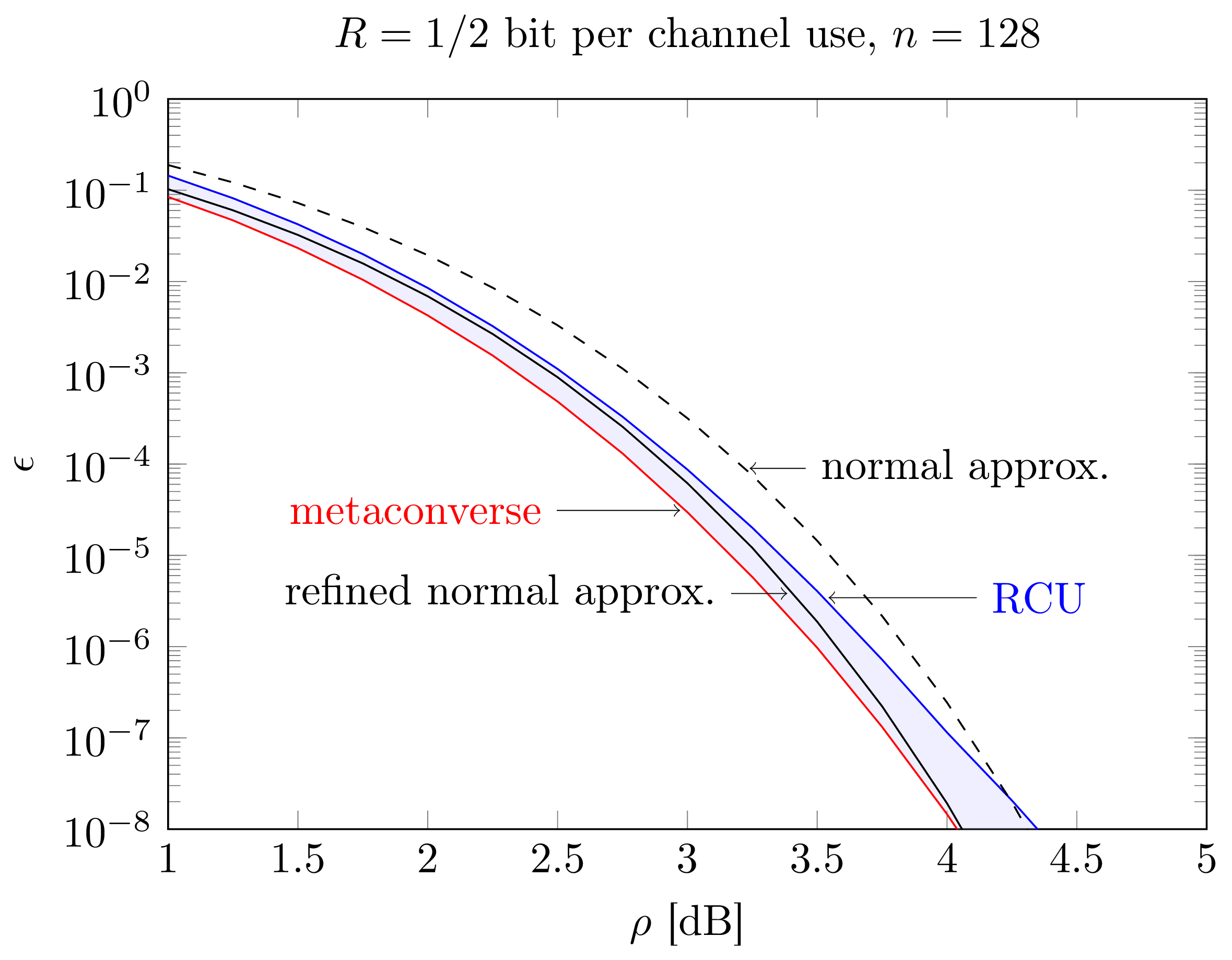
Figure 3.6: Normal approximation vs. finite-blocklength upper and lower bounds on \(\epsilon^*(n,R)\) as a function of the SNR (dB) for \(R=1/2\) bits per channel use and \(n=128\).
So, at least for the scenario considered in Fig. 3.6, the normal approximation is accurate.
When can we expect this to be the case? Roughly speaking, when deriving (3.21), we approximated \[ Q\left(\frac{C-R}{\sqrt{V/n}}\right) + \frac{\mathrm{c}}{\sqrt{n}} = \epsilon \]
where \(\mathrm{c}\) is a constant, with \[ Q\left(\frac{C-R}{\sqrt{V/n}}\right) \approx \epsilon. \]
This approximation is obviously inaccurate when \(Q\bigl((C-R)/\sqrt{V/n}\bigr) \ll c/\sqrt{n}\). This may occur if \(R\ll C\) in which case the \(Q(\cdot)\) may take very small value. It may also occur when \(n\) is small. We illustrate this issue in Figure 3.7 below.
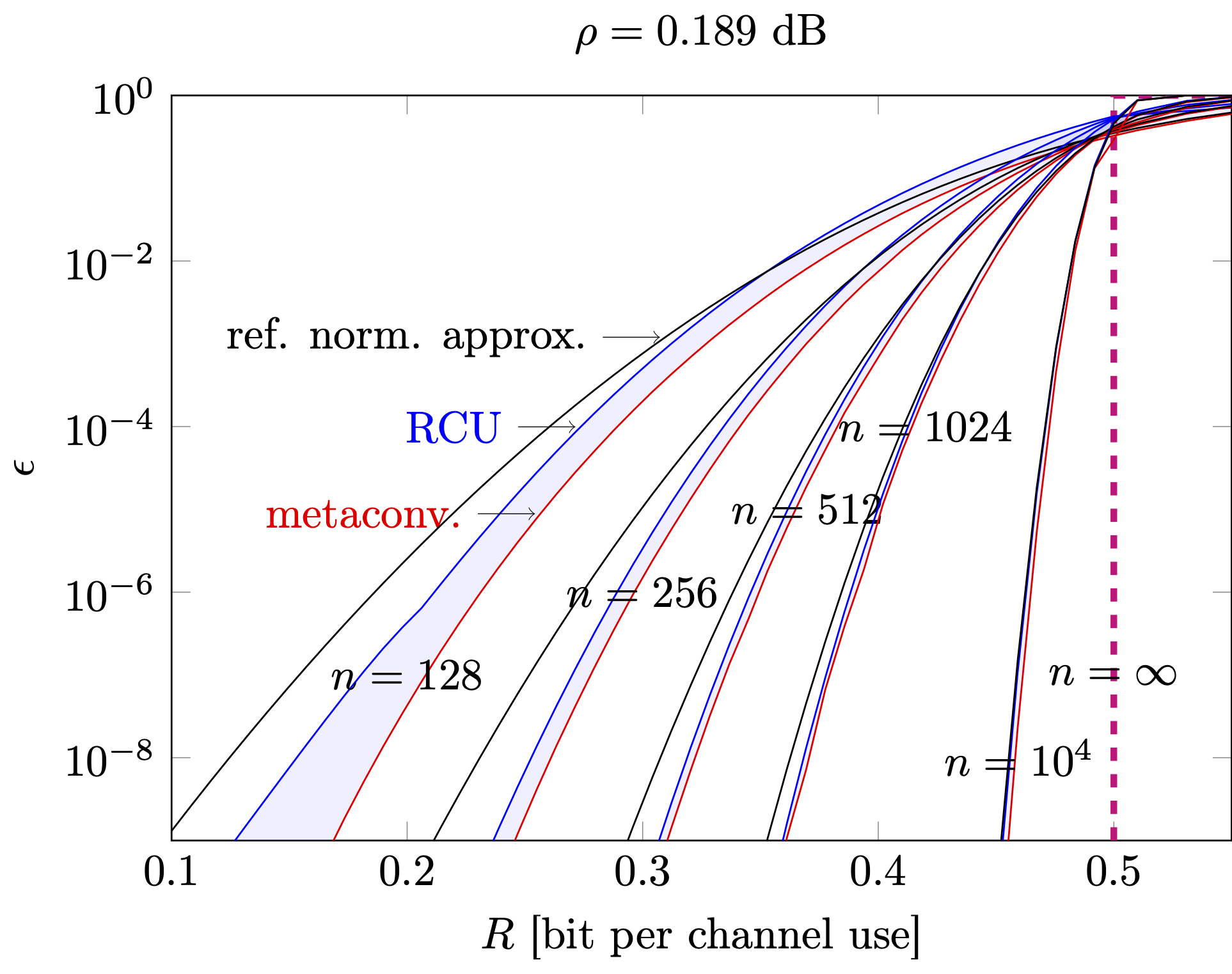
Figure 3.7: Normal approximation vs finite-blocklength upper and lower bounds on \(\epsilon^*(n,R)\) as a function of the rate \(R\) for different values of the blocklength \(n\)
Here, we assume \(\rho=0.189\) dB, for which \(C=0.5\) bits per channel use, and evaluate the tightest achievability and converse bounds available together with the refined normal approximation for different values of the rate \(R\) measured in bits per second. As shown in the figure, the normal approximation loses accuracy as the gap between \(R\) and \(C\) increases and this is particularly problematic for small blocklengths.
To summarize, the normal approximation may be inaccurate when the packets are short, and the selected rate is significantly smaller than the channel capacity, a choice that is unavoidable if one wants to achieve low error probabilities at low SNR values. This is a scenario that is relevant for the ultra-reliable low-latency communication (URLLC) use case recently introduced in 5G. Hence, we conclude that for the URLLC scenario, the use of the normal approximation to predict system performance and perform system design may be questionable.
3.6 Performance of practical error-correcting codes
How close do actual error-correcting codes perform to the bounds just discussed? This questions has been analyzed in many recent papers in the literature. Here, we present some of the results reported in [11]. Please consult this reference for more details about the families of codes discussed here as well as for additional results pertaining some of the codes selected in 5G.
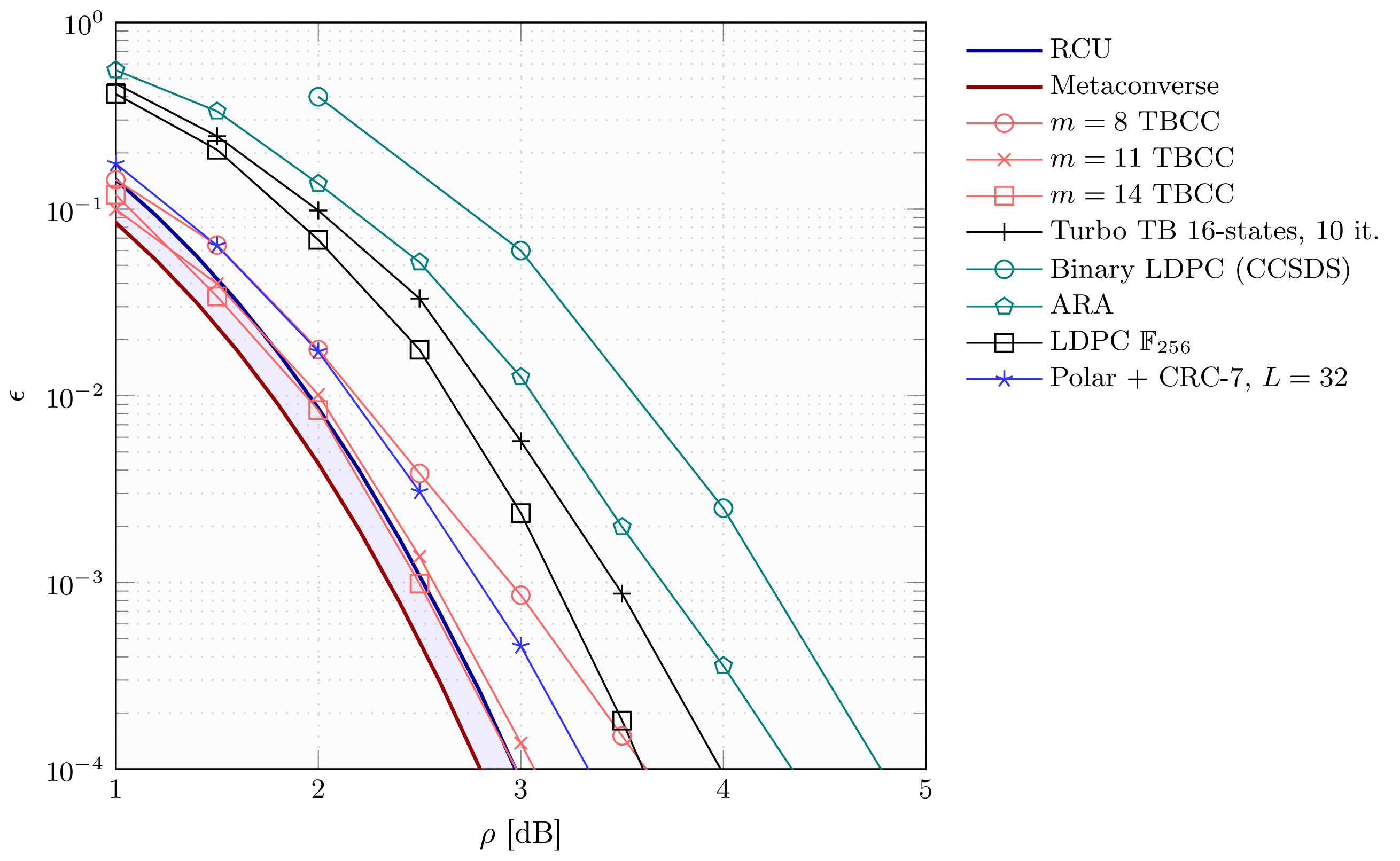
Figure 3.8: Error probability vs. SNR in dB for selected families of channel codes. In the figure, \(k=64\) and \(n=128\)
In Figure 3.8, we plot the RCU and metaconverse bounds for the case \(k=64\) and \(n=128\) as well as the performance of selected classes of codes. As shown in the figure, tail-biting convolutional codes (TBCC) of sufficiently large memory (\(m=14\)) perform very close to the bounds. Modern short codes such as turbo codes and low-density parity-check (LDPC) codes perform worse at these very short blocklengths. In the figure, we reported the performance of the binary LDPC code selected by the Consultative Committee for Space Data Systems (CCSDS) as error-correcting code for the satellite command, as well as the ones of an accumulate-repeat-accumulate (ARA) LDPC code, and a turbo code based on 16-state component recursive convolutional codes. As shown in the figure, better performance (at the cost of an increased decoding complexity) can be obtained with a nonbinary LDPC code over \(\mathbb{F}_{256}\). Finally, one can achieve performance similar to the ones of TBCCs by using a polar code with successive-cancellation list-decoding (with list size \(L=32\)) combined with an outer CRC code of length \(7\).
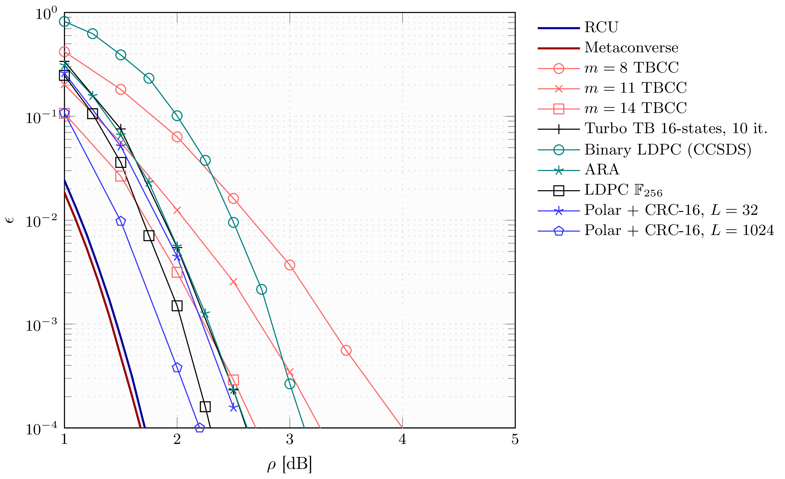
Figure 3.9: Error probability vs. SNR in dB for selected families of channel codes. In the figure, \(k=256\) and \(n=512\)
In Figure 3.9, we consider the case \(k=256\) and \(n=512\). For this scenario, the performance of the TBCCs are not as satisfactory. Indeed, as expected, without further increasing the memory of the constituent convolutional codes, the performance of TBCCs degrade as the blocklength increases. On the contrary, modern short codes have better performance, which is again expected. The best performance in the figure is achieved by a polar code with list-cancellation decoding and list size \(L=1024\), which exhibits a gap of around \(0.5\) dB to the nonasymptotic bounds when \(\epsilon=10^{-4}\).
References
[1] Y. Polyanskiy, H. V. Poor, and S. Verdú, “Channel coding rate in the finite blocklength regime,” IEEE Trans. Inf. Theory, vol. 56, no. 5, pp. 2307–2359, May 2010.
[3] C. E. Shannon, “A mathematical theory of communication,” Bell Syst. Tech. J., vol. 27, pp. 379–423 and 623–656, 1948.
[4] W. Yang, A. Collins, G. Durisi, Y. Polyanskiy, and H. V. Poor, “Beta-beta bounds: Finite-blocklength analog of the golden formula,” IEEE Trans. Inf. Theory, vol. 64, no. 9, pp. 6236–6256, Sep. 2018.
[5] A. Martinez and A. Guillén i Fàbregas, “Saddlepoint approximation of random–coding bounds.” San Diego, CA, U.S.A., Feb. 2011.
[6] R. G. Gallager, Information theory and reliable communication. New York, NY, U.S.A.: Wiley, 1968.
[7] J. Font-Segura, G. Vazquez-Vilar, A. Martinez, A. Guillén i Fàbregas, and A. Lancho, “Saddlepoint approximations of lower and upper bounds to the error probability in channel coding.” Princeton, NJ, Mar. 2018.
[8] Y. Polyanskiy and Y. Wu, Lecture notes on information theory. 2019.
[9] S. Verdú and T. S. Han, “A general formula for channel capacity,” IEEE Trans. Inf. Theory, vol. 40, no. 4, pp. 1147–1157, Jul. 1994.
[10] W. Feller, An introduction to probability theory and its applications, vol. II. New York, NY, USA: Wiley, 1971.
[11] M. C. Coşkun et al., “Efficient error-correcting codes in the short blocklength regime,” Physical Communication, Mar. 2019.